Explore ACR AI-LAB™ Ecosystem, Demonstrations, Commercial Participation and Community resources.
Federated Learning
FL enables data from multiple institutions to be used for training artificial intelligence (AI) models without data leaving institutional firewalls. If you are interested in joining together with other healthcare organizations to create robust AI models through AI-LAB, please sign up to learn more.
Working with ACR, members of the American Academy of Ophthalmology (AAO) have developed use cases involving AI models in the ophthalmic domain for AI-LAB. These include models for automated detection of stages of diabetic retinopathy, different types of retinal findings, glaucoma, and infectious keratitis using a variety of imaging modalities. The AAO is grateful for this multi-disciplinary collaboration with ACR to include ophthalmic images into AI-LAB, and future efforts will include expansion of use cases and data sources.
AI LAB™ Ecosystem
The paper provides an outline and framework for the decisions, infrastructure, and steps
involved in bringing AI into your organization. We encourage all interested parties to
review the framework, including radiologists, data scientists and others in the
radiology community with an interest in AI technology.
The ACR Data Science Institute has developed the ACR AI-LAB™, a data science toolkit designed to democratize AI by empowering radiologists to develop algorithms at their own institutions, using their own patient data, to meet their own clinical needs.
Select a page
Define
Annotate
Create
Evaluate
Run
Publish
Assess
Challenges
Define
Welcome to the ACR AI-LAB™ Define. Browse defined AI use cases, comment on published use cases, and submit a new use case for review.
Instructions
1.Browse defined AI use cases
2.Search, filter, or sort through all of the use cases
3.Click on the use case name under the USE CASE column to comment on a published use case.
4.Click on REQUEST TO DRAFT A USE CASE under the REQUEST column to request to draft a use case that is not yet published.
5.Click on SUBMIT A NEW USE CASE and fill out the form to submit a new AI use case for the ACR to review.
Tutorial
Annotate
Welcome to the ACR AI-LAB™ Annotate. Within each use case, you can annotate multiple scans to develop a data set.
Instructions
1. Select a use case.
2. Select a data set to annotate.
3. Use the image viewing tools to examine the scan.
4. Classify each image by selecting one of the categories.
5. Click NEXT to save your annotation and view the next scan.
6. Click FINISH to finish annotating and return to the home page.
Annotate
Annotate Tutorial
My Annotations
Welcome to the ACR AI-LAB™ My Annotations. Annotate at least 100 of the 5,000 studies to use to build your own breast density classification model.
Instructions
1. Use the image viewing tools to examine the scan.
2. Classify each image by selecting one of the categories.
3. Click SAVE AND CONTINUE to save your annotation and view the next scan.
4. Click SKIP to skip a study. You can always go back to review your skipped studies by clicking on the first dropdown in the upper left corner.
5. View your annotated studies by clicking on the second dropdown in the upper left corner. Change your annotation by selecting a new classification and clicking SAVE AND CONTINUE.
6. Click FINISH to finish annotating and return to the leaderboard. You can return at any time to continue annotating.
My Annotations Tutorial
If you experience any issues during the challenge, please let us know by emailing ailabsupport@acr.org.
Run
Welcome to the ACR AI-LAB™ Run. You can run a model and see the prediction by using a prepopulated image or by uploading your own image.
Instructions
Select an AI use case.
Select a model to run.
Click MORE DETAIL to view more information about the model.
Select a prepopulated image.
Click RUN PREDICTION to view the model’s output.
Click RESET or select another prepopulated image to run another prediction.
Inference
Run Tutorial
Report Text Generation
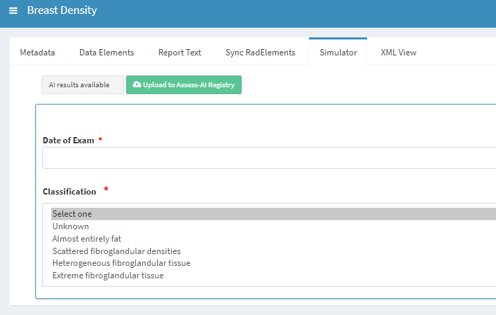
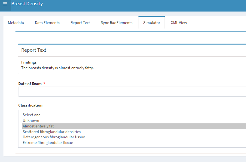
Step 1: Define-AI generates CDEs for a specific use case.
arrow_downward
Step 2: An Assist Module is created for each Define-AI use case which encodes CDEs and associated Report Text as XML
arrow_downward
Step 3: The Assist module can be represented in any UI such as:
Simulator
Radiology Report
Viewer
arrow_downward
Step 4: When the algorithm generates output, the associated Report Text is also generated. The text can be customized to local preference (e.g., can be blank if result is negative).
Publish
Welcome to the ACR AI-LAB™ Publish. You can publish a model you designed on the Create page to a destination like an AI marketplace.
Instructions
Select an AI use case.
If there are no available models, go to the create page, create a model, and save it.
Select a destination to publish your model to.
Click PUBLISH. This will send your model to the destination.
Assess
Welcome to the ACR AI-LAB™ Assess. You can assess the performances of all deployed models.
Instructions
Select an AI use case.
To view just one model at a time, select a model from the drop down list.
Terminology
Kappa Score
Statistic that measures the agreement between two raters that classify items into mutually exclusive categories and takes into account the probability of random agreement.
If two raters are in complete agreement, then the kappa score could be close to 1. If two raters are in complete disagreement, then the kappa score could be close to 0 or even negative if they are agreeing less than the probability of random agreement.
Confusion Matrix
A table that is used to display the performance of a classification model on a test data set as compared to the ground truth. Each square has a unique row and column combination. The square in row 1 and column 2 says that the ground truth classified those test data points as category 1 but the classification model classified those same test data points as category 2. All of the squares along the diagonal of the table display the number of test cases when the ground truth and classification model are in agreement. All squares off the diagonal represent any disagreement between the ground truth and classification model; the further away from the diagonal, the larger the disagreement. If there is complete agreement between the ground truth and classification model, then all of the off diagonal squares will be zero. If there is complete disagreement between the ground truth and classification model, then all of the diagonal squares will be zero.
Binary Threshold
Change the minimum probability threshold value required to classify the study as the positive class. If the probability that a study is in the positive class is greater than or equal to the threshold value, then the study is classified as positive. A threshold of 0.75 requires that the model be 75% sure that the study is in the positive class in order for it to be classified as positive. Whereas a threshold of 0.1 requires that the model only be 10% sure that the study is in the positive class in order for it to be classified as positive. Moving the threshold slider changes the statistics calculated for the specific data element.
Confusion Matrix
A table that is used to display the performance of a classification model on a test data set as compared to the ground truth. Each square has a unique row and column combination. The square in row 1 and column 2 says that the ground truth classified those test data points as category 2 but the classification model classified those same test data points as category 1. All of the squares along the diagonal of the table display the number of test cases when the ground truth and classification model are in agreement. All squares off the diagonal represent any disagreement between the ground truth and classification model; the further away from the diagonal, the larger the disagreement. If there is complete agreement between the ground truth and classification model, then all of the off diagonal squares will be zero. If there is complete disagreement between the ground truth and classification model, then all of the diagonal squares will be zero.
Kappa Score
Statistic that measures the agreement between two raters that classify items into mutually exclusive categories and takes into account the probability of random agreement.
If two raters are in complete agreement, then the kappa score could be close to 1. If two raters are in complete disagreement, then the kappa score could be close to 0 or even negative if they are agreeing less than the probability of random agreement.
AUC Score
(Area Under the the Receiver Operating Characteristic (ROC) Curve or AUC, also known as the C-statistic) Performance measurement for classification problems that measures how well a model separates categories. An AUC score close to 1 means that the model is good at separating categories; it classifies 0s as 0s and 1s as 1s. An AUC score close to 0 means that the model is separating into opposite categories; it classifies 0s as 1s and 1s as 0s. An AUC score close to 0.5 means that the model is no better at separating categories than random chance.
Sensitivity
Statistic that measures the ability of a binary classification model to correctly identify the positive (present) cases. It is the ratio of true positives (both the radiologist and model classify the case as positive) to ground truth positives (all cases the radiologist classifies as positive). Also commonly referred to as true positive rate. A model with 100% sensitivity identifies all positive cases and has few false negatives. However, sensitivity does not factor in false positives.
Specificity
Statistic that measures the ability of a binary classification model to correctly identify the negative (absent) cases. It is the ratio of true negatives (both the radiologist and model classify the case as negative) to ground truth negatives (all cases the radiologist classifies as negative). Also commonly referred to as selectivity or true negative rate. A model with 100% specificity identifies all negative cases and has few false positives. However, specificity does not factor in false negatives.
Linnear Kappa
Statistic that measures the agreement between two raters that classify items into mutually exclusive categories and takes into account the probability of random agreement. If two raters are in complete agreement, then the kappa score could be close to 1. If two raters are in complete disagreement, then the kappa score could be close to 0 or even negative if they are agreeing less than the probability of random agreement.
Scatterplot of Volumes
A scatterplot that compares the size of the predicted volumes to the size of the ground truth volumes. If all of the points fall on the dotted line, then the size of the predicted volumes is equal to the size of the ground truth volumes. If the points fall below the dotted line, then the model is generally predicting smaller volumes than the ground truth. If the points fall above the dotted line, then the model is generally predicting larger volumes.
Bland-Altman Plot
The Bland-Altman plot shows the agreement between two quantitative measurements. The x-axis shows the average of the two measures and the y-axis shows the difference between the two measures. The mean difference is shown as a solid horizontal line and indicates the bias between the two measurements. If mean difference line is at 0, then on average, there is no bias between the measurements. Additionally, there are two more solid horizontal lines indicating the ±2 standard deviations of the mean difference (about 95% of the points should fall between the two lines). The Bland-Altman plot is helpful in discovering biases in quantitative measurements.
Mean Dice Coefficient
Statistic that measures the average similarity between two sets (segmentations or bounding boxes for example). A dice coefficient close to 1 signifies the sets are very similar; there is a large overlap between the predicted set and the ground truth set. A dice coefficient close to 0 signifies the sets are very dissimilar; there is very little overlap. The dice coefficient is positively correlated with Intersection over Union statistic. Generally, the mean dice coefficient will be higher for larger ground truth volumes (the radiologist's segmentation is large compared to the original image) than for smaller ground truth volumes (the radiologist's segmentation is small).
Mean Average Precision
Statistic that measures the Average Precision of the volumes at different Intersection over Union thresholds. Average Precision is the ratio of true positives to true positives, false positives, and false negatives. Average Precision is not concerned with true negatives. A Mean Average Precision close to 1 indicates that on average, there is a large overlap of predicted volumes and ground truth volumes. A Mean Average Precision close to 0 indicates that the predicted volumes are generally missing the ground truth volumes. Because this statistic is for volumes and not classes, another statistic (Intersection over Union) is used to calculate which volumes are labeled true positives. An IoU Threshold (T) is used as the minimum IoU required to label a volume as a true positive. For example, if the IoU Threshold is set to T=0.5, then a predicted volume that overlaps 75% with the ground truth (IoU = 0.75 which is greater than T) is considered a true positive. However, a predicted volume that overlaps 49% with the ground truth (IoU = 0.49 which is less than T) is considered a false negative. The Mean Average Precision statistic is the mean Average Precision of all images over the range of IoU Thresholds.
Mean Intersection over Union
Statistic that measures the average ratio of the intersection (volume of overlap) and the union (combined volumes) of the predicted and ground truth volumes. If the prediction matches the ground truth exactly, then the overlap and the union would be the same, resulting in an Intersection over Union (IoU)=1. If the prediction completely misses the ground truth, then the overlap is zero, resulting in an Intersection over Union (IoU)=0. The Mean IoU is the average intersection over union of all the bounding boxes.
Random Sampling
Sample the studies randomly, in the distribution they are found in the original dataset.
Positives Only
Sample only the positive cases in the training dataset.
Equal Class Ratios
Sample the studies so that each class is represented equally – 25% almost entirely fat,
25% scattered fibroglandular densities etc.
Sigmoid Focal Loss
Sigmoid Focal Loss reduces the importance of easy cases and increases the importance of the more difficult cases. This is very helpful when using imbalanced datasets - when there are a lot more of one class than the other. Sigmoid Focal Loss allows the model to focus on the more difficult cases.
Predicted Probability over Time
Predicted Probability over Time uses the Study Date field in the DICOM header to monitor the model's predictions over time. The y-axis is the probability that the case is in the positive class (present) according to the model. The horizontal line indicates the Binary Threshold; the model classifies all cases above the threshold line as positive (present) and all cases below as negative (absent). In instances where the radiologist disagrees with the model's classification, the color will indicate if it is a false positive or a false negative.
RoC Curve
Receiver operating Characteristic (RoC) Curve shows the trade-off between sensitivity and specificity for all thresholds. The blue circle will move depending on the Binary Threshold. A curve that is close to diagonal indicates that the model is no better than random chance. A curve that hugs the top left corner indicates good model performance. The area under the RoC curve is the AUC score.
Evaluate
Welcome to the ACR AI-LAB™ Evaluate. Within each use case, you can test multiple models on the same test data set and compare the performances.
Instructions
Select an AI use case.
Select a validation data set.
Click on the models you want to evaluate, you may click on more than one.
Click EVALUATE MODELS to view the test results.
Click SHOW MODELS to change your selections.
Kappa Score
Statistic that measures the agreement between two raters that classify items into mutually exclusive categories and takes into account the probability of random agreement.
If two raters are in complete agreement, then the kappa score could be close to 1. If two raters are in complete disagreement, then the kappa score could be close to 0 or even negative if they are agreeing less than the probability of random agreement.
AUC Score
(Area under the curve of the Receiver operating characteristic) Performance measurement for classification problems that measures how well a model separates categories. An AUC score close to 1 means that the model is good at separating categories; it classifies 0s as 0s and 1s as 1s. An AUC score close to 0 means that the model is separating into opposite categories; it classifies 0s as 1s and 1s as 0s. An AUC score close to 0.5 means that the model is no better at separating categories than random chance.
Confusion Matrix
A table that is used to display the performance of a classification model on a test data set as compared to the ground truth. Each square has a unique row and column combination. The square in row 1 and column 2 says that the ground truth classified those test data points as category 1 but the classification model classified those same test data points as category 2. All of the squares along the diagonal of the table display the number of test cases when the ground truth and classification model are in agreement. All squares off the diagonal represent any disagreement between the ground truth and classification model; the further away from the diagonal, the larger the disagreement. If there is complete agreement between the ground truth and classification model, then all of the off diagonal squares will be zero. If there is complete disagreement between the ground truth and classification model, then all of the diagonal squares will be zero.
Create
Welcome to the ACR AI-LAB™ Create. Within each use case, you can design your own AI models and train, test, and run them on data sets.
Instructions
Define the problem.
Select a body area.
Select a modality.
Select an AI use case.
Prepare the data.
Select the training data set.
Select the Augmentation.
Click START PREPROCESSING to prepare the data.
Configure your model.
Select the model architecture.
Select the data sampling method.
Select the model loss function.
Select if the model is pre-trained or not.
Select if the model has early stopping or not.
Click TRAIN AND TEST to train and test your model.
Click RUN PREDICTION to view the model’s prediction.
Repeat the process to create another model. You can continue to add models to your screen.
Click REMOVE to remove a model from your screen.
Terminology
Training Dataset Size
The size of the training dataset can affect the accuracy of the model.
In general, the model will be more accurate as the training dataset size increases.
Data Set
The dataset that contains the prepared images that you train the model with.
If no data sets are listed, you will need to prepare them first.
Augmentation
Apply additional transformations, such as rotations, flips, or stretching, to images input to the network.
None: Do not transform images.
Random Flips/Rotations: Add random flips and rotations to the scans before the model sees them.
Architectures
Structure of the neural network.
ResNet: Type of architecture developed in 2015 for the ImageNet Large Scale Visual Recognition
Challenge that introduced skipped connections between layers and won first place in image classification,
detection, and localization.
VGGNet: Type of architecture developed in 2014 for the ImageNet Large Scale Visual Recognition Challenge
that won first place on image localization.
InceptionNet: Type of architecture whose innovation was to attempt to process information at different spatial scales.
It also used new methods to make neural networks "deeper" (more complex) while still learning broad, generalizable
concepts about its chosen task.
DenseNet: Type of architecture whose innovation in neural networks allowed them to maintain high levels of complexity and
classification ability, while greatly reducing the computational time and memory required to classify a single case.
Architecture Videos
Sampling Methods
Technique for selecting the studies that the model sees at each training step.
Equal Class Ratios: Sample the studies so that each class is represented equally – 25% almost entirely fat,
25% scattered fibroglandular densities etc.
Random Sampling: Sample the studies randomly, in the distribution they are found in the original dataset.
{{option.text}}
Loss Functions
How the model knows what to learn
Mean Absolute Error
Treat all successes differently depending on confidence, treat all failures differently depending on confidence.
If the model got the right category and was very confident in the choice, then it was a large success. If the model got the right category and was not confident in the choice, then it was a small success. If the model got the wrong category and was not confident in the choice, then it was a small failure. If the model got the wrong category and was very confident in the choice, then it was a large failure.
Assume that the distance between the categories is the same.
Categorical Cross-Entropy
Treat all successes differently depending on confidence, treat all failures equally.
If the model got the right category and was very confident
in the choice, then it was a large success. If the model got the right category and was not confident in the choice, then it was a small success.
If the model got the wrong category, then it was a failure and all failures are treated the same.
Mean-Squared Error
Treat all successes differently depending on confidence, treat all failures differently depending on confidence.
If the model got the right category and was very confident in the choice, then it was a large success. If the model got the right category and was not confident in the choice, then it was a small success. If the model got the wrong category and was not confident in the choice, then it was a small failure. If the model got the wrong category and was very confident in the choice, then it was a large failure.
Heavily penalize large failures and assume that the distance between the categories is the same.
Loss function Videos
Pretraining
Whether or not the model has been trained on a different task before training on a new task
Random Initialization: Randomly start the model, it has not been pretrained on another task.
Pretrained Weights (ImageNet): Start with a pretrained model that was previously trained to classify natural images,
such as photos of cars, dogs, and buildings.
Batch Size
The number of training examples the model learns from during a single step. If the batch size is too small, it can lead to chaotic training because the model doesn't see enough examples at once. If the batch size is too large, the training may fail due to memory constraints of the server. If the training keeps failing, try the smallest batch size possible and increase until the memory limit is exceeded.
Initial Learning Rate
How much the model should change while learning from the training data. A learning rate that is too small can lead to long training times and could cause the model to get 'stuck'. A learning rate that is too high can lead to chaotic training because the model is changing too much.
Improvement Interval
Number of epochs the model will wait for improvement before early stopping. If early stopping is True, then the model will continue to train for a minimum improvement interval. If no improvement is made, then the model will stop training early. If there is improvement, the interval restarts. If early stopping is False, the model will not stop training early.
Early Stopping
If there is early stopping, the model will stop learning once its performance is no longer improving.
Performance Metric
The metric being used to measure the performance of the algorithm.
Mean Average Precision
AUC
Sigmoid Focal Loss
Confusion Matrix
Kappa
AUC
Sensitivity
Specificity
Kappa Score
Statistic that measures the agreement between two raters that classify items into mutually exclusive categories and takes into account the probability of random agreement.
If two raters are in complete agreement, then the kappa score could be close to 1. If two raters are in complete disagreement, then the kappa score could be close to 0 or even negative if they are agreeing less than the probability of random agreement.
AUC Score
(Area under the curve of the Receiver operating characteristic) Performance measurement for classification problems that measures how well a model separates categories. An AUC score close to 1 means that the model is good at separating categories; it classifies 0s as 0s and 1s as 1s. An AUC score close to 0 means that the model is separating into opposite categories; it classifies 0s as 1s and 1s as 0s. An AUC score close to 0.5 means that the model is no better at separating categories than random chance.
Confusion Matrix
A table that is used to display the performance of a classification model on a test data set as compared to the ground truth. Each square has a unique row and column combination. The square in row 1 and column 2 says that the ground truth classified those test data points as category 1 but the classification model classified those same test data points as category 2. All of the squares along the diagonal of the table display the number of test cases when the ground truth and classification model are in agreement. All squares off the diagonal represent any disagreement between the ground truth and classification model; the further away from the diagonal, the larger the disagreement. If there is complete agreement between the ground truth and classification model, then all of the off diagonal squares will be zero. If there is complete disagreement between the ground truth and classification model, then all of the diagonal squares will be zero.
Overfitting
Epochs
Pre-processing
Confusion Matrix Details vs. Accuracy
Kappa
Create Tutorial: Part1
Create Tutorial: Part2
Train My Models
Welcome to the ACR AI-LAB™ Train My Models. Design and train models using the data annotated on My Annotations. Submit models to the leaderboard.
Train My Models Tutorial
Instructions
Prepare the data.
Select your annotated data as the training data set. You need at least 100 annotations in order to train.
Select the Augmentation.
Configure your model.
Select the model architecture.
Select the data sampling method. You may only choose equal sampling if you have at least 10 annotations of each classification.
Select the model loss function.
Select to begin with a pre-trained model or a brand new model.
Select if the model has early stopping or not.
Choose the maximum number of epochs. If early stopping is true, then your model might not reach this maximum.
Click TRAIN AND TEST to send your model to ACR's GPUs for training and testing.
Click CANCEL to cancel a model's training. A model training can only be cancelled if it is queued or in progress.
Repeat the process to create another model.
Click SUBMIT to submit a model to the challenge leaderboard. You may submit as many models as you want before the end of the challenge but only your most recent submission will appear on the leaderboard.
Terminology
Training Dataset Size
The size of the training dataset can affect the accuracy of the model.
In general, the model will be more accurate as the training dataset size increases.
Augmentation
Apply additional transformations, such as rotations, flips, or stretching, to images input to the network.
None: Do not transform images.
Random Flips/Rotations: Add random flips and rotations to the scans before the model sees them.
Prepared Dataset
.......
Architectures
Structure of the neural network.
ResNet: Type of architecture developed in 2015 for the ImageNet Large Scale Visual Recognition
Challenge that introduced skipped connections between layers and won first place in image classification,
detection, and localization.
VGGNet: Type of architecture developed in 2014 for the ImageNet Large Scale Visual Recognition Challenge
that won first place on image localization.
InceptionNet: Type of architecture whose innovation was to attempt to process information at different spatial scales.
It also used new methods to make neural networks "deeper" (more complex) while still learning broad, generalizable
concepts about its chosen task.
DenseNet: Type of architecture whose innovation in neural networks allowed them to maintain high levels of complexity and
classification ability, while greatly reducing the computational time and memory required to classify a single case.
Architecture Videos
Sampling Methods
The ratio of each class that the model sees at each training step
Equal Class Ratios: Sample the studies so that each class is represented equally – 25% almost entirely fat,
25% scattered fibroglandular densities etc.
Random Sampling: Sample the studies randomly, in the distribution they are found in the original dataset.
Loss Functions
How the model knows what to learn
Mean Absolute Error
Treat all successes differently depending on confidence, treat all failures differently depending on confidence.
If the model got the right category and was very confident in the choice, then it was a large success. If the model got the right category and was not confident in the choice, then it was a small success. If the model got the wrong category and was not confident in the choice, then it was a small failure. If the model got the wrong category and was very confident in the choice, then it was a large failure.
Assume that the distance between the categories is the same.
Categorical Cross-Entropy
Treat all successes differently depending on confidence, treat all failures equally.
If the model got the right category and was very confident
in the choice, then it was a large success. If the model got the right category and was not confident in the choice, then it was a small success.
If the model got the wrong category, then it was a failure and all failures are treated the same.
Mean-Squared Error
Treat all successes differently depending on confidence, treat all failures differently depending on confidence.
If the model got the right category and was very confident in the choice, then it was a large success. If the model got the right category and was not confident in the choice, then it was a small success. If the model got the wrong category and was not confident in the choice, then it was a small failure. If the model got the wrong category and was very confident in the choice, then it was a large failure.
Heavily penalize large failures and assume that the distance between the categories is the same.
Loss function Videos
Pretraining
Whether or not the model has been trained on a different task before training on a new task
Random Initialization: Randomly start the model, it has not been pretrained on another task.
Pretrained Weights (ImageNet): Start with a pretrained model that was previously trained to classify natural images,
such as photos of cars, dogs, and buildings.
Early Stopping
If there is early stopping, the model will stop learning once its performance is no longer improving.
Epochs
The number of times the model learns from the training dataset.
Kappa Score
Statistic that measures the agreement between two raters that classify items into mutually exclusive categories and takes into account the probability of random agreement.
If two raters are in complete agreement, then the kappa score could be close to 1. If two raters are in complete disagreement, then the kappa score could be close to 0 or even negative if they are agreeing less than the probability of random agreement.
AUC Score
(Area under the curve of the Receiver operating characteristic) Performance measurement for classification problems that measures how well a model separates categories. An AUC score close to 1 means that the model is good at separating categories; it classifies 0s as 0s and 1s as 1s. An AUC score close to 0 means that the model is separating into opposite categories; it classifies 0s as 1s and 1s as 0s. An AUC score close to 0.5 means that the model is no better at separating categories than random chance.
Confusion Matrix
A table that is used to display the performance of a classification model on a test data set as compared to the ground truth. Each square has a unique row and column combination. The square in row 1 and column 2 says that the ground truth classified those test data points as category 1 but the classification model classified those same test data points as category 2. All of the squares along the diagonal of the table display the number of test cases when the ground truth and classification model are in agreement. All squares off the diagonal represent any disagreement between the ground truth and classification model; the further away from the diagonal, the larger the disagreement. If there is complete agreement between the ground truth and classification model, then all of the off diagonal squares will be zero. If there is complete disagreement between the ground truth and classification model, then all of the diagonal squares will be zero.
Overfitting
Epochs
Pre-processing
Confusion Matrix Details vs. Accuracy
Kappa
Confusion Matrix Tutorial
If you experience any issues during the challenge, please let us know by emailing ailabsupport@acr.org.
Crowdsourcing Contest
Welcome to the ACR AI-LAB™ BREAST DENSITY CROWDSOURCING CONTEST. Annotate as many breast density scans as you can over the course of the ACR's annual meeting.
Instructions
Use the image viewing tools to examine the scan.
Classify each image by selecting one of the categories.
Click SKIP if you do not want to annotate that specific scan.
Click NEXT to save your annotation and view the next scan.
Click FINISH to finish annotating. You may return at any time.
The number at the top right of the page denotes the total number of images you have annotated.
Overview
Participation Tutorial
Registration Tutorial
Instructions
Prepare the data.
Select the Usecase
Select the training data set.
Choose Prep for Annotation
Choose Prep for Model Creation
Click Prepare Data to process the dataset for Annotation and Model Creation
Use Cases
Select the use case for which you would like to prepare the data for.
Data Set
Select the data set that contains the images that you would like to prepate.
If no data sets are listed, you will need to create them first in Data Manager.
Prep for Annotation
Select to convert the Dicom images on the dataset into png images for annotation purposes.
Prep for Model Creation
Select to convert the Dicom images in the dataset into Numpy objects for model creation.
Crowdsourcing Contest
Welcome to the ACR AI-LAB™ BREAST DENSITY CROWDSOURCING CONTEST. Annotate as many breast density scans as you can over the course of the ACR's annual meeting.
Instructions
Use the image viewing tools to examine the scan.
Classify each image by selecting one of the categories.
Click SKIP if you do not want to annotate that specific scan.
Click NEXT to save your annotation and view the next scan.
Click FINISH to finish annotating. You may return at any time.
The number at the top right of the page denotes the total number of images you have annotated.
Overview
Participation Tutorial
Registration Tutorial
Residency Mammography Challenge
Welcome to the ACR AI-LAB™ Residency Mammography Challenge.
Instructions
Click MY ANNOTATIONS to annotate at least 100 of the 5,000 breast density studies. Your annotations will be used for the training data set. You can compare your overall annotation distribution with that of a DMIST reader in the confusion matrix on this page but will not be able to see the DMIST reader annotations on an image level.
Click TRAIN MY MODELS to design your own AI model by adjusting hyperparameters and training on your own annotated data.
Send in your design for training, also known as a job, to ACR's GPUs.
Submit a model to the leader board to compare your test results with other models. The test data set will be using DMIST reader annotations as ground truth.
You may submit as many models as you want before the end of the challenge but only your most recent submission will appear on the leaderboard. The leaderboard is ranked by kappa scores on the test results. At the end of the challenge, all submissions will be judged against a final test data set so the leaderboard is not necessarily indicative of who could win.